Plot the pdfs as violins
Arguments
- x
A
crestObjgenerated by either thecrest.calibrate,crest.reconstructorcrestfunctions.- climate
Climate variables to be used to generate the plot. By default all the variables are included.
- taxanames
A list of taxa to use for the plot (default is all the recorded taxa).
- col
A vector of colours that will be linearly interpolated to give a unique colour to each taxon.
- ylim
The climate range to plot the pdfs on. Default is the full range used to fit the
pdfs(x$modelling$xrange)- save
A boolean to indicate if the diagram should be saved as a pdf file. Default is
FALSE.- filename
An absolute or relative path that indicates where the diagram should be saved. Also used to specify the name of the file. Default: the file is saved in the working directory under the name
'violinPDFs.pdf'.- width
The width of the output file in inches (default 7.48in ~ 19cm).
- height
The height of the output file in inches (default 3in ~ 7.6cm per variables).
- as.png
A boolean to indicate if the output should be saved as a png. Default is
FALSEand the figure is saved as a pdf file.- png.res
The resolution of the png file (default 300 pixels per inch).
Value
A table with the climate tolerances of all the taxa
Examples
if (FALSE) { # \dontrun{
data(crest_ex_pse)
data(crest_ex_selection)
reconstr <- crest.get_modern_data(
pse = crest_ex_pse, taxaType = 0,
climate = c("bio1", "bio12"),
selectedTaxa = crest_ex_selection, dbname = "crest_example"
)
reconstr <- crest.calibrate(reconstr,
geoWeighting = TRUE, climateSpaceWeighting = TRUE,
bin_width = c(2, 20), shape = c("normal", "lognormal")
)
} # }
## example using pre-saved reconstruction obtained with the previous command.
data(reconstr)
ranges <- plot_violinPDFs(reconstr, save=FALSE, ylim=c(5,35),
taxanames=c(reconstr$inputs$taxa.name[c(2,4,5,1)]),
col=c('darkblue', 'firebrick3'))
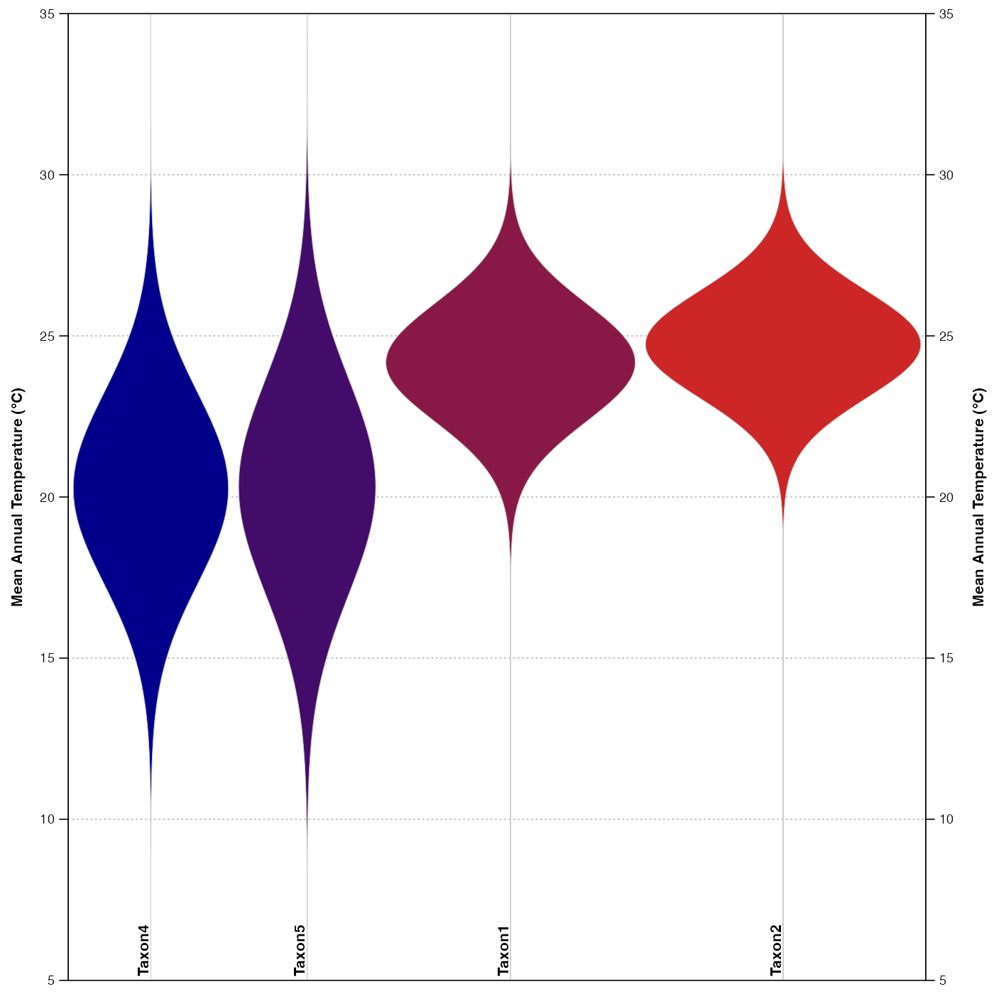 lapply(ranges, head)
#> $`Range = 50%`
#> bio1_tol_inf bio1_tol_sup bio1_range
#> Taxon1 23.00601 25.33066 2.324649
#> Taxon2 23.64729 25.81162 2.164329
#> Taxon4 18.35671 22.20441 3.847695
#> Taxon5 18.11623 22.52505 4.408818
#>
#> $`Range = 95%`
#> bio1_tol_inf bio1_tol_sup bio1_range
#> Taxon1 20.68136 27.73547 7.054108
#> Taxon2 21.56313 27.97595 6.412826
#> Taxon4 14.50902 25.97194 11.462926
#> Taxon5 13.86774 26.85371 12.985972
#>
lapply(ranges, head)
#> $`Range = 50%`
#> bio1_tol_inf bio1_tol_sup bio1_range
#> Taxon1 23.00601 25.33066 2.324649
#> Taxon2 23.64729 25.81162 2.164329
#> Taxon4 18.35671 22.20441 3.847695
#> Taxon5 18.11623 22.52505 4.408818
#>
#> $`Range = 95%`
#> bio1_tol_inf bio1_tol_sup bio1_range
#> Taxon1 20.68136 27.73547 7.054108
#> Taxon2 21.56313 27.97595 6.412826
#> Taxon4 14.50902 25.97194 11.462926
#> Taxon5 13.86774 26.85371 12.985972
#>