The CREST method (Climate REconstruction SofTware) is a climate reconstruction technique that combines presence-only occurrence data with modern climatologies to estimate the conditional responses of a given set of taxa to a variable of interest [1-2]. The combination of these responses is used to estimate past climate probabilities. The CREST method is especially useful for reconstructing climate conditions in regions where climate reconstructions are scarce or fragmented, such as tropical forests or remote mountain ranges. This broad applicability has made it invaluable for studies aiming to understand past climate variability and its impacts on ecosystems worldwide.
Fossil data used in CREST often includes pollen grains, foraminifers, or plant macrofossils collected from sediment cores or archaeological sites. To illustrate the conceptual background of CREST, we will consider fossil pollen data, as these are great, ubiquitous climate proxies. In CREST, climate reconstructions are based on the combination of the climate preferences and tolerances of the taxa observed in the fossil record. Probability Density Functions (PDFs) are used to describe the range of climatic conditions a taxon is likely to prefer, based on statistical analysis of its modern occurrence. For instance, PDFs can show how likely it is to observe cacti along an aridity gradient range.
One specific characteristic of pollen data (and many other proxies) is their limited taxonomical resolution. Usually, they cannot be identified at the species level but at a higher level (sub-genus to family level), which complexifies the modelling of the pollen-climate responses [3]. The PDFs are thus estimated in one or two steps based on the nature of the proxy being studied. In simple cases, where fossils can be identified at the species level (e.g. foraminifers, plant macrofossils), the PDFs are defined by unimodal and parametric functions (e.g. normal or log-normal distributions depending on the nature of the studied variable, see [1-2] for a more detailed discussion). These distributions are described by parameters such as a mean and standard deviation. CREST estimates these values using modern climate data linked to the species’ observed presence (Fig. 1), each being weighted as an inverse function of its abundance in the study area. This correction removes the influence of the heterogeneously distributed modern climate space and ensures that the optimum exhibited by the PDF reflects the true climatic preference of the species, rather than the modern abundance of a given climate value [4-5].
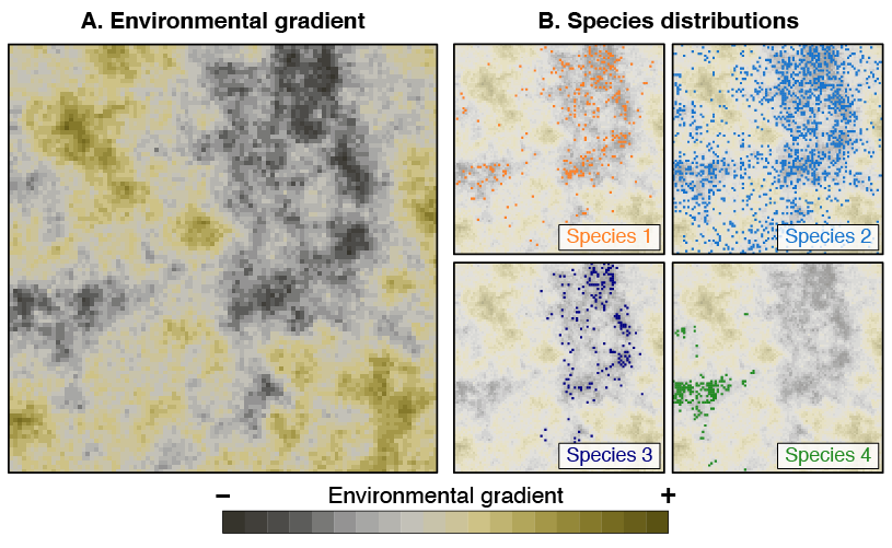
Fig. 1: This figure illustrates how CREST uses modern observation data to infer PDFs. (left) Climate variable to reconstruct (e.g. mean annual temperature). (Right) Four distinct plant taxa living in that region and having a preference for the darker climates (e.g. a preference for colder climates). These four species produce indistinguishable pollen grains and, therefore, define a ‘pollen type’. This example is based on pseudo-data.
A second step is necessary to create the taxon-climate probabilistic link when the fossils cannot be identified at the species level (e.g. pollen grains identified at the genus or family level). Initially, a parametric PDF is created for each species that produces similar pollen grains. These individual PDFs are then combined into a higher-order PDF to represent the entire pollen type (Fig. 2). CREST does not impose specific shapes on the pollen PDFs, allowing them to reflect the full range of climate preferences exhibited by different species. It is worth noting that the process can be used with incomplete distribution data because CREST uses parametric functions to define the species PDFs. Reconstructions from modern [1] and fossil [6-9] data suggest that robust PDFs can still be obtained from truncated geographical distributions, provided that the full range of the climatic tolerance of the species is well covered in the climate space [10].
By linking fossil data to climatic variables through PDFs, CREST has been successfully used to reconstruct temperature and precipitation patterns in diverse ecosystems, from African savannahs to Andean cloud forests, from relatively short (millennial) 50 million year old records .
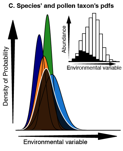
Fig. 2: Climate responses of the four plant species presented on Fig. 1 (coloured curves). Their individual responses are combined together to create the response of the pollen taxon in black. The histogram inset represents the distribution of the climate space available (white) and which part of this climate space is occupied by at least one species (in black).
Once estimated for all taxa, the PDFs for the taxa identified in a sample are multiplied together, each with a weight derived from the observed percentages. Since relative abundances, different production rates and taphonomy are important factors influencing the fossil assemblage observed, direct percentages cannot be used directly. To account for biases in fossil data, CREST transforms the raw percentages, ensuring more accurate climate reconstructions. In CREST, the transformation is performed on a taxon basis by normalising the raw percentages by the average of the percentages of all the samples where the taxon is observed (i.e. the zeros are excluded). A value higher (lower) than one suggests that the climate at the time of deposition was more (less) favourable (i.e. closer to the taxon’s climate optimum) than the average climate in which the taxon has been observed during the studied period.
The multiplication of PDFs results in a likelihood distribution along the climate gradient, from which climate estimates and uncertainties can be derived (Fig. 3). More technical details about the different parameterisations of the method can be obtained from the original publications (1-2).
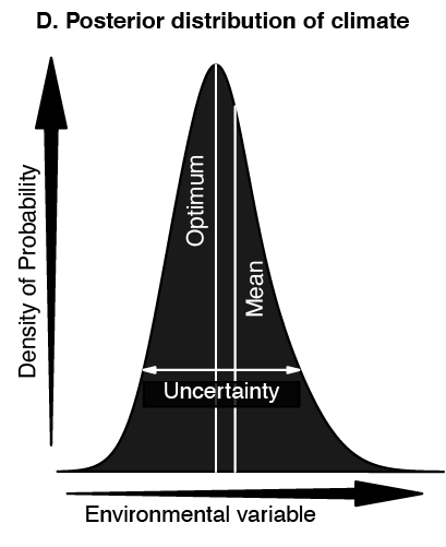
Fig. 3: Likelihood distribution conditioned by the existence of certain fossil taxa observed with certain proportions. This distribution can be simplified to single number, such as the mean or the mode/optimum (i.e. the most likely) probability.
In summary, CREST is a statistical tool that links fossil data to climatic variables through Probability Density Functions (PDFs). By providing meaningful uncertainty estimates alongside reconstructions, CREST’s probabilistic framework ensures robust data for addressing critical research questions, such as the drivers of long-term climate shifts or regional ecosystem resilience.
References
[1] Chevalier, M., Cheddadi, R., Chase, B.M., 2014. CREST (Climate REconstruction SofTware): a probability density function (PDF)-based quantitative climate reconstruction method. Clim. Past 10, 2081–2098. doi:10.5194/cp-10-2081-2014.
[2] Chevalier, M., 2022. crestr an R package to perform probabilistic climate reconstructions from palaeoecological datasets. Clim. Past doi:10.5194/cp-18-821-2022.
[3] Chevalier, M., 2019. Enabling possibilities to quantify past climate from fossil assemblages at a global scale. Global and Planetary Change, 175, pp. 27–35. doi:10.1016/j.earscirev.2020.103384.
[4] Kühl, N., Gebhardt, C., Litt, T., Hense, A., 2002. Probability Density Functions as Botanical-Climatological Transfer Functions for Climate Reconstruction. Quat. Res. 58, 381–392. doi:10.1006/qres.2002.2380.
[5] Bray, P.J., Blockley, S.P.E., Coope, G.R., Dadswell, L.F., Elias, S.A., Lowe, J.J., Pollard, A.M., 2006. Refining mutual climatic range (MCR) quantitative estimates of palaeotemperature using ubiquity analysis. Quat. Sci. Rev. 25, 1865–1876. doi:10.1016/j.quascirev.2006.01.023.
[6] Chevalier, M., Chase, B.M., 2015. Southeast African records reveal a coherent shift from high- to low-latitude forcing mechanisms along the east African margin across last glacial–interglacial transition. Quat. Sci. Rev. 125, 117–130. doi:10.1016/j.quascirev.2015.07.009.
[7] Chevalier, M., Chase, B.M., 2016. Determining the drivers of long-term aridity variability: a southern African case study. J. Quat. Sci. 31, 143–151. doi:10.1002/jqs.2850.
[8] Lim, S., Chase, B.M., Chevalier, M., Reimer, P.J., 2016. 50,000 years of climate in the Namib Desert, Pella, South Africa. Palaeogeogr. Palaeoclimatol. Palaeoecol. 451, 197–209. doi:10.1016/j.palaeo.2016.03.001.
[9] Cordova, C.E., Scott, L., Chase, B.M., Chevalier, M., 2017. Late Pleistocene-Holocene vegetation and climate change in the Middle Kalahari, Lake Ngami, Botswana. Quat. Sci. Rev. 171, 199–215. doi:10.1016/j.quascirev.2017.06.036.
[10] Chevalier, M., Davis, B.A.S., Heiri, O., Seppä, H., Chase, B.M., Gajewski, K., Lacourse, T., Telford, R.J., Finsinger, W., Guiot, J., Kühl, N., Maezumi, S.Y., Tipton, J.R., Carter, V.A., Brussel, T., Phelps, L.N., Dawson, A., Zanon, M., Vallé, F., Nolan, C., Mauri, A., de Vernal, A., Izumi, K., Holmström, L., Marsicek, J., Goring, S., Sommer, P.S., Chaput, M. and Kupriyanov, D., 2020. Pollen-based climate reconstruction techniques for late Quaternary studies. Earth-Science Reviews, 210, pp. 103384. doi:10.1016/j.earscirev.2020.103384.