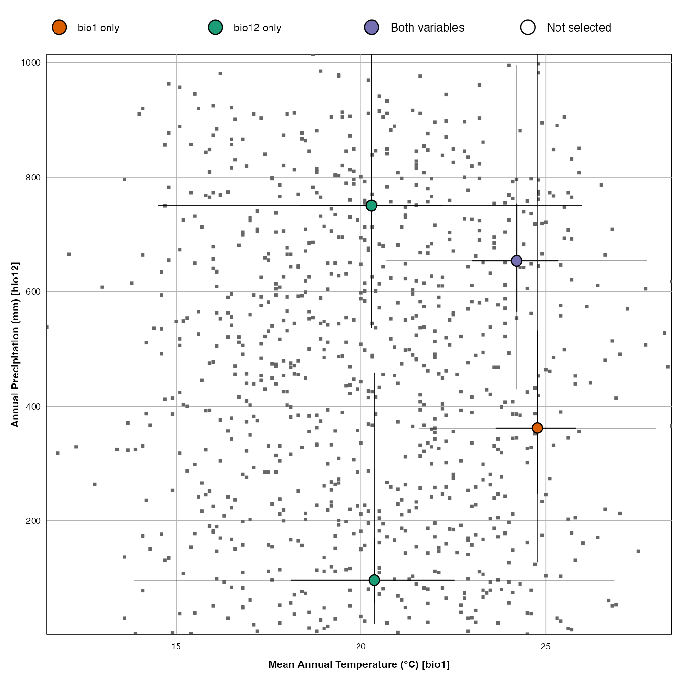
Plot the pdf optima and uncertainty ranges in a climate biplot
Source:R/plot.scatterPDFS.R
plot_scatterPDFs.RdPlot the pdf optima and uncertainty ranges in a climate biplot
plot_scatterPDFs(
  x,
  climate = x$parameters$climate[1:2],
  taxanames = x$input$taxa.name,
  uncertainties = x$parameters$uncertainties,
  xlim = range(x$modelling$climate_space[, climate[1]]),
  ylim = range(x$modelling$climate_space[, climate[2]]),
  add_modern = FALSE,
  save = FALSE,
  filename = "scatterPDFs.pdf",
  width = 5.51,
  height = 5.51,
  as.png = FALSE,
  png.res = 300
)
Arguments
- x
A
crestObjgenerated by either thecrest.calibrate,crest.reconstructorcrestfunctions.- climate
Names of the two climate variables to be used to generate the plot. By default plot. By default the first two variables are included.
- taxanames
A list of taxa to use for the plot (default is all the recorded taxa).
- uncertainties
A (vector of) threshold value(s) indicating the error bars that should be calculated (default are the values stored in x).
- xlim,
ylim The climate range to plot the data. Default is the full range of the observed climate space.
- ylim
the y limits of the plot.
- add_modern
A boolean to add the location and the modern climate values to the plot (default
FALSE).- save
A boolean to indicate if the diagram should be saved as a pdf file. Default is
FALSE.- filename
An absolute or relative path that indicates where the diagram should be saved. Also used to specify the name of the file. Default: the file is saved in the working directory under the name
'violinPDFs.pdf'.- width
The width of the output file in inches (default 7.48in ~ 19cm).
- height
The height of the output file in inches (default 3in ~ 7.6cm per variables).
- as.png
A boolean to indicate if the output should be saved as a png. Default is
FALSEand the figure is saved as a pdf file.- png.res
The resolution of the png file (default 300 pixels per inch).
Value
A table with the climate tolerances of all the taxa
Examples
if (FALSE) { # \dontrun{
  data(crest_ex_pse)
  data(crest_ex_selection)
  reconstr <- crest.get_modern_data(
    pse = crest_ex_pse, taxaType = 0,
    climate = c("bio1", "bio12"),
    selectedTaxa = crest_ex_selection, dbname = "crest_example"
  )
  reconstr <- crest.calibrate(reconstr,
    geoWeighting = TRUE, climateSpaceWeighting = TRUE,
    bin_width = c(2, 20), shape = c("normal", "lognormal")
  )
} # }
## example using pre-saved reconstruction obtained with the previous command.
data(reconstr)
dat <- plot_scatterPDFs(reconstr, save=FALSE,
                 taxanames=c(reconstr$inputs$taxa.name[c(2,4,5,1)]))

dat
#> $`Range = 50%`
#>        bio1_tol_inf bio1_tol_sup bio1_range bio12_tol_inf bio12_tol_sup
#> Taxon2     23.64729     25.81162   2.164329     247.49499      531.4629
#> Taxon4     18.35671     22.20441   3.847695     669.53908      841.4830
#> Taxon5     18.11623     22.52505   4.408818      57.31463      169.3387
#> Taxon1     23.00601     25.33066   2.324649     565.33066      752.9058
#>        bio12_range
#> Taxon2    283.9679
#> Taxon4    171.9439
#> Taxon5    112.0240
#> Taxon1    187.5752
#>
#> $`Range = 95%`
#>        bio1_tol_inf bio1_tol_sup bio1_range bio12_tol_inf bio12_tol_sup
#> Taxon2     21.56313     27.97595   6.412826     127.65531     1021.2425
#> Taxon4     14.50902     25.97194  11.462926     536.67335     1047.2946
#> Taxon5     13.86774     26.85371  12.985972      20.84168      458.5170
#> Taxon1     20.68136     27.73547   7.054108     429.85972      995.1904
#>        bio12_range
#> Taxon2    893.5872
#> Taxon4    510.6212
#> Taxon5    437.6754
#> Taxon1    565.3307
#>
dat
#> $`Range = 50%`
#> bio1_tol_inf bio1_tol_sup bio1_range bio12_tol_inf bio12_tol_sup
#> Taxon2 23.64729 25.81162 2.164329 247.49499 531.4629
#> Taxon4 18.35671 22.20441 3.847695 669.53908 841.4830
#> Taxon5 18.11623 22.52505 4.408818 57.31463 169.3387
#> Taxon1 23.00601 25.33066 2.324649 565.33066 752.9058
#> bio12_range
#> Taxon2 283.9679
#> Taxon4 171.9439
#> Taxon5 112.0240
#> Taxon1 187.5752
#>
#> $`Range = 95%`
#> bio1_tol_inf bio1_tol_sup bio1_range bio12_tol_inf bio12_tol_sup
#> Taxon2 21.56313 27.97595 6.412826 127.65531 1021.2425
#> Taxon4 14.50902 25.97194 11.462926 536.67335 1047.2946
#> Taxon5 13.86774 26.85371 12.985972 20.84168 458.5170
#> Taxon1 20.68136 27.73547 7.054108 429.85972 995.1904
#> bio12_range
#> Taxon2 893.5872
#> Taxon4 510.6212
#> Taxon5 437.6754
#> Taxon1 565.3307
#>